Code & Tools
Hands-on tutorial: Granulometric analysis of 21 cm tomography
Hands-on tutorial: Granulometric analysis of 21 cm tomography
This is a hands-on tutorial on the granulometric analysis of 21 cm tomographic data (image or datacube). In-depth discussion on the astrophysical application is described in Kakiichi et al. (2017). This tutorial aims at describing the practical aspects and the python script of the method.Background: algebra of shapes
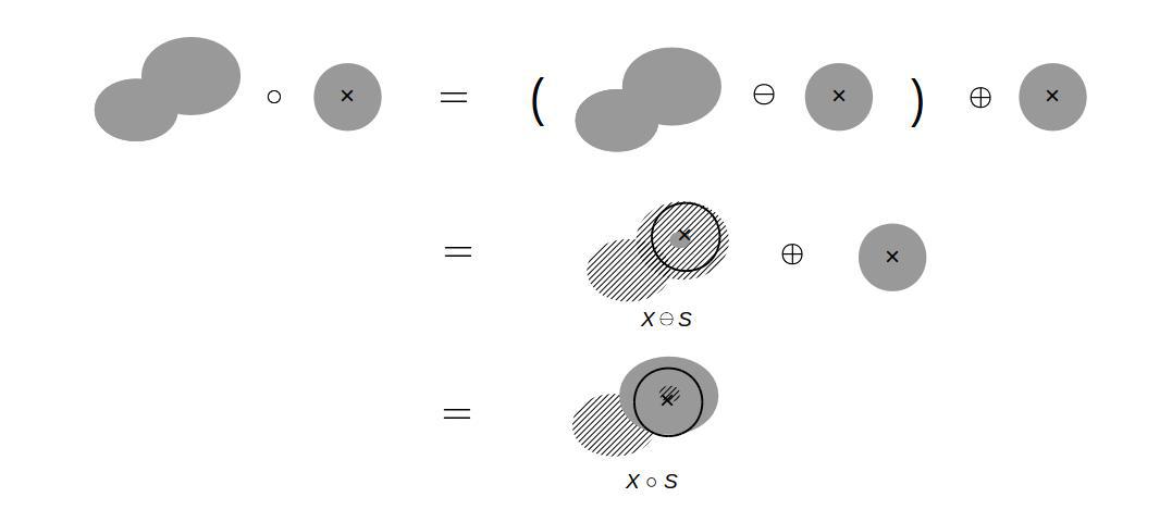
First of all, we need to set up a mathematical tool: algebra of shapes. The followings are the well-defined operations in mathematical morphology. The Minkowski addition (dilation) is given by the union of a binary field, X, and a structuring element, S, as the structuring element is moved on the binary field. The diagram below illustrates how this Minkowski sum operation works.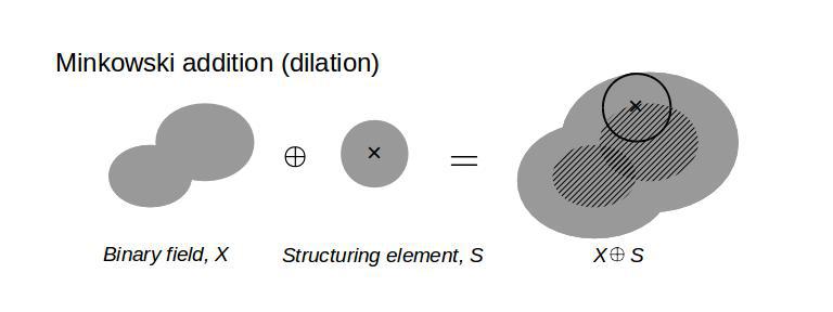
Python scripts
Example image: excursion set of a Gaussian random field
import numpy as np
import scipy.ndimage

Ng=300          # number of cells
smoothing=5     # smoothing scale in pixels
threshold=0.05  # threshold defining the excursion sets of a random field

random_field=np.random.randn(Ng,Ng)
binary_field=scipy.ndimage.gaussian_filter(random_field,sigma=smoothing) > threshold
Thanks to python scipy package (scipy.ndimage, see morphology), the above morphological operations can be implemented very easily (almost one line!). First, we
need define the shape of a structuring element, which is used to analyse an image. We take a sphere of radius n in pixels.
def sphere(n):
    struct = np.zeros((2 * n + 1, 2 * n + 1))
    x, y = np.indices((2 * n + 1, 2 * n + 1))
    mask = (x - n)**2 + (y - n)**2 <= n**2
    struct[mask] = 1
    return struct.astype(np.bool)
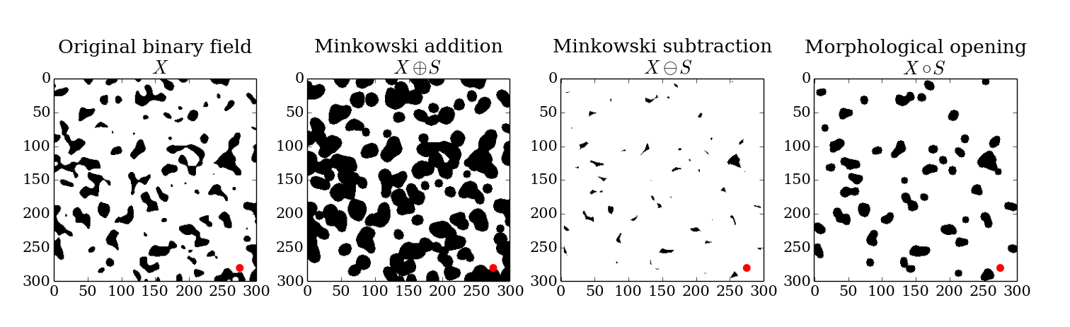
Then, the Minkowski addition, subtraction, and morphological opening of the binary field with the structuring element are simply,
n=5 # radius of a spherical structuring element in pixels
# Minkowski addition (dilation)
dilation=scipy.ndimage.binary_dilation(binary_field,structure=sphere(n))
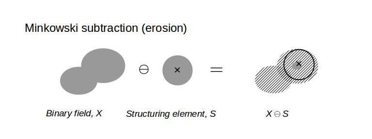
# Minkowski subtraction (erosion)
erosion=scipy.ndimage.binary_erosion(binary_field,structure=sphere(n))
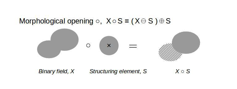
# Morphological opening (sieving)
opening=scipy.ndimage.binary_opening(binary_field,structure=sphere(n))
The results of these morphological operations are show in Figure 4.
Granulometry: size distribution
Granulometry is a method to measure the size distribution of a binary field (2D or 3D) using successive morphological opening operations with varying sizes of a structuring element. An implementation with Python is
# python script to measure the size distribution of
# a binary 2D image or 3D datacube using a granulometric method

def granulometry(data,dim):
    def disk(n):
        struct = np.zeros((2 * n + 1, 2 * n + 1))
        x, y = np.indices((2 * n + 1, 2 * n + 1))
        mask = (x - n)**2 + (y - n)**2 <= n**2
        struct[mask] = 1
        return struct.astype(np.bool)
    def ball(n):
        struct = np.zeros((2*n+1, 2*n+1, 2*n+1))
        x, y, z = np.indices((2*n+1, 2*n+1, 2*n+1))
        mask = (x - n)**2 + (y - n)**2 + (z - n)**2 <= n**2
        struct[mask] = 1
        return struct.astype(np.bool)

    s = max(data.shape)
    area0=float(data.sum())
    area=np.zeros(s/2)
    pixel=range(s/2)
    for n in range(s/2):
        print 'binary opening the data with radius =',n,' [pixels]'
        if dim == 2:
            opened_data=scipy.ndimage.binary_opening(data,structure=disk(n))
        if dim == 3:
            opened_data=scipy.ndimage.binary_opening(data,structure=ball(n))
        area[n]=float(opened_data.sum())
        if area[n] == 0:
            break

    pattern_spectrum=np.zeros(s/2)
    for n in range(s/2-1):
        pattern_spectrum[n]=(area[n]-area[n+1])/area[0]

    return (area,pattern_spectrum,pixel)
Usage
# usage example
dim=2
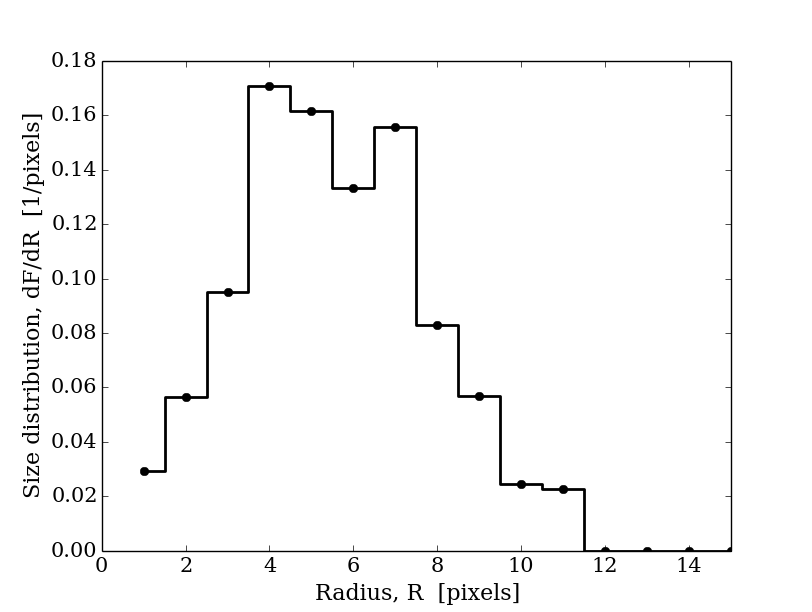
area,dFdR,pixel=granulometry(binary_field,dim)
R=np.array(pixel) # radius of structural element [pixels]
import matplotlib.pyplot as plt
plt.figure()
plt.plot(R[1:], dFdR[1:], 'ko-',linewidth=2,drawstyle='steps-mid')
plt.xlabel('Radius, R [pixels]')
plt.ylabel('Size distribution, dF/dR [1/pixels]')
plt.xlim(0,15)
plt.show()